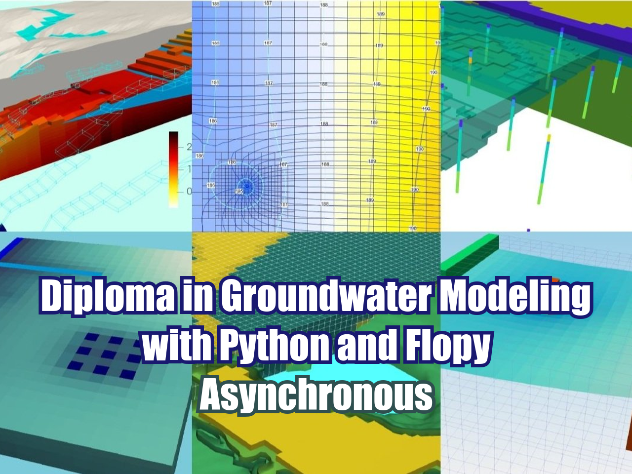
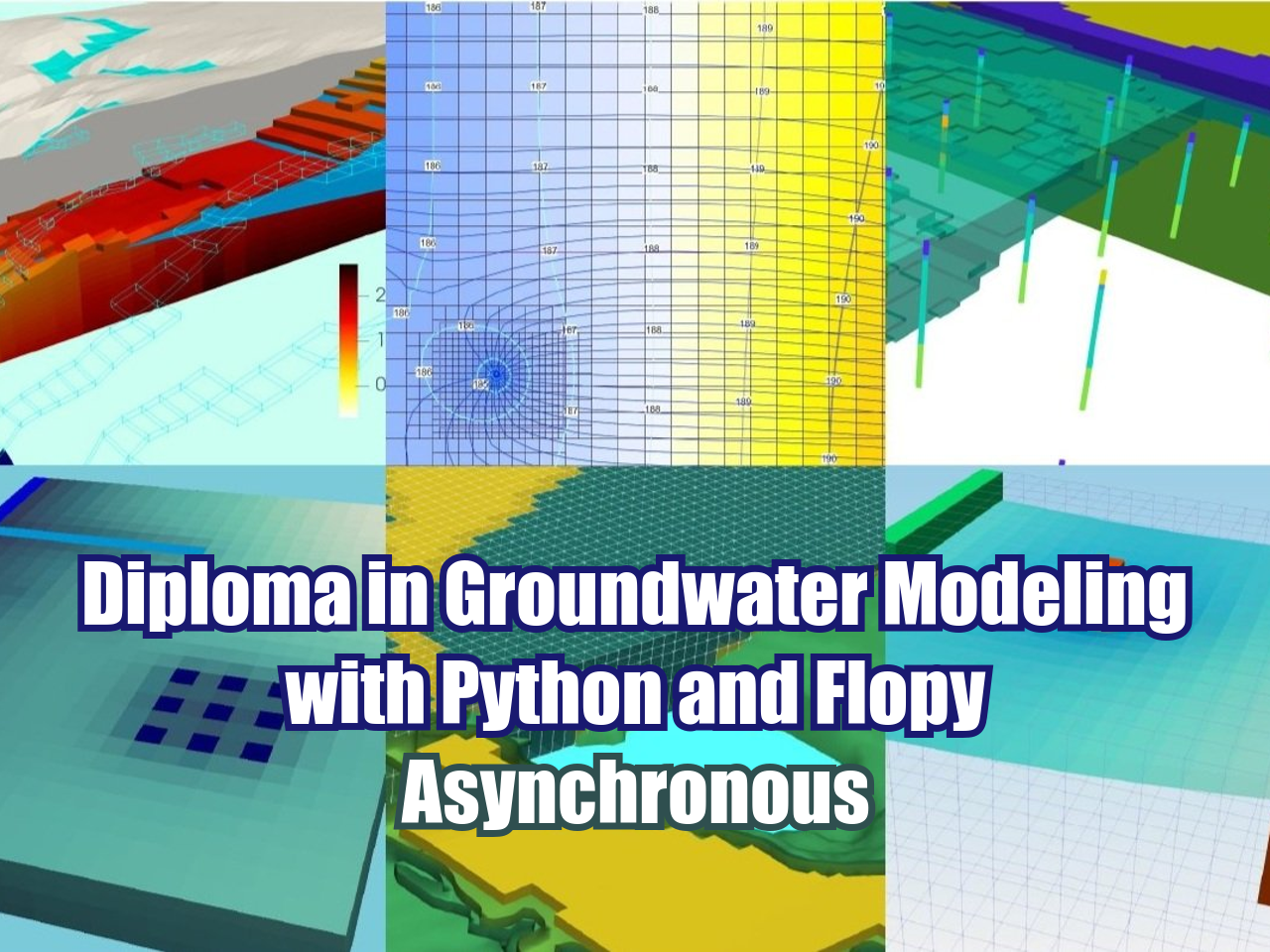
FloPy is the Python library that builds and executes MODFLOW models; this library has been enhanced to provide full support of MODFLOW 6 with most of its recent development is related to functionality for MODFLOW 6, tools to use vector and raster spatial data and common plotting and export functionality.
Python is a simple and powerful programming language; its simplicity is remarkable compared to other programming languages and its power is based on the number of tools available for different areas of study.
We have developed a complete program on groundwater modeling with MODFLOW and FloPy that ranges from the essential topics in Python to applied cases of regional modeling, seawater intrusion and Pest optimization. The program is designed to give the student a methodological approach to learn FloPy based on a series of applied examples coupled by teacher insights and review from the software.
Objectives
The student will reach the following objectives based on a hands-on learning approach through understanding simple to complex concepts:
- Use Python as a tool to import, create, run MODFLOW models
- Develop a knowledge on the most basic concepts of Flopy
- Manage the most popular tools of FloPy library
- Use Flopy on real case escenarios and couple with other Python libraries
Content
The diploma is divided into six modules. The summarized content of every module is described below:
Module 1. Introduction to Python
This course develops the basic concepts of Python programming under Jupyter. Exercises will cover the basic Python data structures, conditional statements, loops coupled with an introduction to array manipulation in Numpy, tabular data management with Pandas and applied exercises with precipitation data.
Session 1: Python data types
Understanding the way Python works and exploring the numerical types together with mathematical operations. Strings and boolean expressions are also reviewed.
- Basic concepts of the Anaconda distribution and Jupyter Lab tools.
- Lexical and syntax analysis.
- Types and objects (strings, list, tuples and dictionaries).
- Expressions and operators.
- Conditions and iterations.
Session 2: Python loops and data structures
A review of the conditional forms and functions in Python with practical examples of creation, indexing and management of lists, tuples, dictionaries and sets.
- Lists.
- Functions.
- Loop with while and for.
- Dictionaries.
Session 3: Numpy for water resources
This session covers the key concepts of multidimensional arrays management with Numpy.
- Numpy array creation
- Operation with numpy arrays
- Indexing and redimension of numpy arrays
Session 4: Data manipulation with Pandas
This session covers the concepts for analyzing, exploring and manipulating data with applied examples.
- Filtering temporal series
- Columns and rows manipulation
- Pandas calculations and groups
- Exporting data
Session 5: Overview to Matplotlib
This session is focused on learning how to use the Matplotlib library that provides blocks to create visualizations for different kinds of data and how to customize them.
- Introduction to Matplotlib.
- Creation of a simple plot using Matplotlib.
- Customizing plots.
- Bar and histogram plots.
- Scatter and 3D scatter plots.
Session 6: Introduction to Geopandas
This session will cover an analysis of flooded areas impact on infrastructure with Python and Geopandas. The exercise will show how Geopandas can manage both the spatial analysis and operation among columns.
- Reading data into Geopandas.
- Working with linestrings and points.
- Spatial operation.
- Plotting data with Folium.
- Clipping and exporting flooded areas.
Module 2: Groundwater modeling with FloPy and MODFLOW-2005
This module deals with the basic concepts of groundwater modeling with Flopy and MODFLOW-2005 and MODFLOW-NWT. The applied cases covered on this module give the student the overall functionality of FloPy with this MODFLOW version.
Session 1: Basic example of a MODFLOW-2005 model creation and simulation with FloPy
This session covers a basic example of model creation, configuration and simulation in Python 3 on a Jupyter Notebook. The example also shows the procedure to import the MODFLOW results done with FloPy in Model Muse.
- Model geometry construction
- Setup of boundary conditions
- Model simulation and head representation
- Format output to be read in Model Muse
Session 2: 2D contaminant transport modeling with MODFLOW-2005, MT3D-USGS and FloPy
This session covers the simulation of a 2D transport model build with FloPy, MODFLOW and MT3D. Model is constructed on a structured grid, boundary conditions are set for steady state flow conditions.
- Definition of temporal and spatial discretizations.
- Setup of boundary conditions for flow and transport.
- Define contaminant sources and transport parameters
- Plot concentration distribution
Session 3: Contaminant transport modeling with remediation schema using MODFLOW-2005, MT3D-USGS and FloPy
This session develops a complete applied case of flow and transport modeling with MODFLOW, MT3D-USDS and FloPy. The study case describes a regional groundwater flow which has a point source with a remediation schema simulated on steady state conditions for flow conditions and transient for transport modeling.
- Configuration of a MODFLOW model with FloPy
- Setting up of spatial and temporal discretization
- Configuration of a MT3D-USGS model with FloPy
- Implementation of advection, dispersion and mass sources
Session 4: Example of particle tracking modeling with MODPATH 7, MODFLOW-2005 and FloPy
MODPATH is a particle tracking post-processing package that computes and displays three-dimensional pathlines based on output from MODFLOW. These pathlines help us to see the expected transport trajectories coming from a specific contaminant source.
This is an applied case of particle tracking with MODPATH 7 on structured grid on MODFLOW-2005.
- Define the flow model data
- Create MODPATH zones, particles and particle groups
- Run flow and particle tracking models
- Plot MODPATH 7 output
Session 5: Determination of flow direction vectors from a MODFLOW-2005 model with Python and Flopy
Groundwater flow direction representation is useful to understand the actual and predicted conditions of the groundwater flow regime. The arrow direction and magnitude give a quick perspective of the main groundwater flow directions and the interconnection between sources and discharge points. This session shows the complete workflow to determine the flow directions from a MODFLOW model done with Model Muse.
- Set a background image for the figure
- Create a MODFLOW model as an object
- Import some geospatial parameters from the model
- Import the output heads
- Create the flow direction vectors
Module 3: Groundwater modeling with FloPy and MODFLOW-6
Particular cases for building and simulating MODFLOW-6 models with Flopy are covered in this module. There is a special focus on dealing with the difference of MODFLOW-6 with other versions and how these differences are reflected on the FloPy commands and tools.
Session 1: Basic example of groundwater modeling with wells and regional flow in with MODFLOW-6 and FloPy
This session shows the complete procedure to setup, run and visualize a basic groundwater model in MODFLOW 6 with FloPy. The model has 2 stress periods, 800 cells, 2 layers with constant heads on the sides to represent regional flow and pumping wells located on different layers.
- Model creation and solver options
- Definition of temporal and spatial discretization
- Definition of hydraulic parameters, initial conditions and boundary conditions
- Model simulation and output representation
Session 2: Basic example of groundwater modeling in MODFLOW-6 and visualization with Paraview and FloPy
Basic example to learn the procedure to build, simulate and represent a MODFLOW 6 model. The example shows an introduction to the model file system on steady state flow conditions. The model is implemented with the following boundary conditions: Drains, Recharge, Wells, and Constant Head and has 30 rows, 24 columns and 3 layers.
- Define model and spatial discretization
- Apply hydraulic parameters and initial conditions
- Setup of boundary conditions
- Export results as Vtk files
Session 3: Modeling aquifer response to pumping with MODFLOW-6
Aquifer response to pumping is one of the most popular interactions between
humans and the groundwater flow regimen. FloPy and Jupyter together can
provide new and powerful ways to analyze the hydrogeological response to a
pumping test on a numerical model.
- Definition of simulation names and model names
- Temporal and spatial discretization
- Definition of hydraulic conductivities and storage
- Interactive sliders to go back and forth on the time steps
Session 4: Groundwater modeling with triangular mesh with MODFLOW-6 and FloPy
FloPy has tools and functionalities for triangular mesh generation. This session covers the complete process to create a triangular mesh with the utilities from FloPy and incorporate it to a MODFLOW 6 model. The model is simulated and results are represented as colored mesh and contour lines.
- Define model domain and drain location
- Triangle mesh generation
- Configuration of the triangular discretization DISV package
- Model simulation and output data representation
Module 4: Regional and geospatial modeling with FloPy
This module covers applied examples of groundwater modeling at regional scale with the use of geospatial libraries in Python. The module also explores the FloPy to set coordinate info and other spatial features.
Session 1: Regional groundwater modeling on andean basins with MODFLOW and FloPy
An applied case of regional modeling on the Angascancha basin with FloPy and MODFLOW NWT. The model is build on steady state flow conditions and output representation has been done with FloPy and Matplotlib tools.
- Open and read raster files
- Define spatial discretization
- Write files of the MODFLOW model and run simulation
- Model grid and heads representation
Session 2: Develop a full geospatial groundwater model with MODFLOW-2005 and FloPy
FloPy, the Python library to build and simulate MODFLOW models, has tools to georeference the model grid even with rotation options. The workflow is kind of explicit, meaning that the modeler need a medium knowledge of Python and FloPy tools. This applied case shows the whole procedure to create a fully geospatial groundwater with MODFLOW and FloPy.
- Define refinement areas and build spatial / temporal discretization
- Definition of the GRIDGEN object
- RCH, EVT, WEL and GHB boundary condition setup
- Model output visualization
Session 3: MODFLOW-2005 infrastructure tunnel model review, simulation and output representation
This session covers the complete procedure to read, simulate and output analysis of a MODFLOW NWT model of a infraestructure tunnel development with time. The applied case include a discussion and review of the different tools available in FloPy and the interaction with QGIS.
- Display model discretization and hydraulic parameters
- Export model features to shapefile format
- Read water budgets per time step as pandas dataframe
- Spatial water head representation
- Create animation over stress periods
Module 5: FloPy utilities for MODFLOW
The FloPy library has tools and utilities for exporting data and plot results. This module has applied cases of head representation and gridded and vector data export.
Session 1: Export MODFLOW-6 properties, boundary conditions and head contours as Shapefiles with FloPy
Sometime there is a need to represent model properties and output in another platforms as GIS. FloPy comes with several tools to export not only the head equipontential at a given layer but also to export the different model parameters as a gridded vector file. This session will show the complete overview of the export options from FloPy.
- Open a regional model
- Setup the coordinate info
- Explore and visualize the different packages
- Export gridded vector data
- Export contour lines
Session 2: How to export 3d model MODFLOW-6 features and heads in Vtk format
FloPy has an export tool to export Structured, Vertex and Unstructured Grid based models to Vtk format to be displayed inside Jupyter and on another software as Paraview. This session covers an applied example of Vtk file generation from a structured grid model in MODFLOW 2005 and its further visualization in Paraview.
- Export model top and bottom
- Export hydraulic parameters and boundary conditions
- Create a Vtk object and export selected data
- Introduction to Vtk visualization in Paraview
Session 03: Export and explore massive MODFLOW-2005 model data with FloPy and NetCDF
Model construction and simulation can produce huge amounts of data. NetCDF is a data format for managing array-oriented scientific data with high performance, Python packages such as Xarray give us a higher degree of functionality when dealing with array data and it is capable to open/read/write NetCDF files. This session covers an applied example of NetCDF creation of from a regional model.
- Open an regional model
- Export model features and output data as NetCDF
- Overview of Xarray package
- Explore and query gridded data with Xarray
Module 6: Seawater intrusion modeling with FloPy
Flopy covers two options for variable density flow: SEAWAT and the BUY package in MODFLOW-6. This module has applied examples for both cases that covers the flow and transport models and the coupling among them…more info.
Session 1: Basic example of saline intrusion modeling with SEAWAT and FloPy
SEAWAT is a model developed by the USGS for the simulation of three-dimensional variable density groundwater flow. This session shows the complete workflow to create and represent a basic example of saline instrusion with SEAWAT and FloPy on a Jupyter Notebook
- Define model dimensions, spatial discretization and hydraulic parameters
- Definition of the flow packages for the SEAWAT model
- Setup of the MT3DMS models and the SEAWAT variable density flow package
- Model results post-processing
Session 2: Seawater intrusion modeling with MODFLOW-6, Model Muse and FloPy
MODFLOW 6 implements the Buoyancy package for the simulation of variable density and seawater intrusion cases. We have developed an applied case seawater intrusion model on a regular geometry model constructed with FloPy for flow and transport.
- Construction of model geometry
- Setup of boundary conditions
- Create auxiliary variable and enable Buy package
- Define transport model, model exchange and run model
- Import and plot results
Session 3: Coupling seawater intrusion with FloPy and MODFLOW-6 and BUY package to a Model Muse project
The groundwater flow model was constructed on Model Muse with two stress periods and a total simulation time of 40 years. The model files are imported with FloPy where the Buy package for variable density flow is implemented together with the transport model.
- Open MF6 and explore packages
- Review of geometry and boundary conditions
- Create auxiliary variable, enable Buy package and define transport model
- Explore the head and concentration results
Module 7. Applied groundwater modeling with FloPy
This module deals with real cases of Flopy application. The example covered on this session covers particular cases on groundwater modeling and give the student the panorama of working with Flopy together with other Python libraries.…more info.
Session 1: How to insert a 3D Geology into a MODFLOW-2005 model with FloPy
This tutorial has an applied example of the implementation of a 3D geological model from a neural network into a groundwater model with determined horizontal discretization and layer thickness. The tutorial covers all the steps for model construction and hydrogeological unit determination with scripts in Python with FloPy and other libraries.
- Definition of area of interest and output grid refinement
- Creation of a model topography
- Apply the lithological model on the UPW package
- Comparisons of the original and translated geological model
Session 2: Sensibility analysis of MODFLOW-6 groundwater models with FloPy and SALib
Sensitivity analysis is referred to the uncertainty analysis in model results from the uncertainties on the model inputs. This session covers an applied case of sensibility analysis over a basic groundwater flow model in MODFLOW 6 with FloPy and SALib libraries.
- Define a MODFLOW6 model as a object
- Python class to modify parameters
- Implementation of SALib to a MODFLOW 6 model
- Result visualization and analysis
Session 3: Effective stress calculation from MODFLOW-NWT groundwater flow model with FloPy
This session covers a full deduction of the effective stress calculation based on the model geometry and an applied example for the effective stress calculation on a hillslope groundwater flow model. The example model was developed in MODFLOW-NWT and Model Muse, whereas the effective stress determination was done with scripts in Python and FloPy.
- Review of the flow model in Model Muse
- Open model and import heads
- Effective stress calculation from heads and geometry
- Export effective stresses as VTKs
Session 4: Tidal water level response on coastal aquifers modeling with MODFLOW-6, FloPy and Timeseries
An “hybrid” approach where a coastal aquifer is built on Model Muse and later imported by FloPy where the boundary conditions that represent the sea elevation is replaced by a time series, new stress periods are inserted, workspace has changed and the model is simulated.
- Redefinition of spatial discretization
- Define timeseries and reassign boundary conditions
- Spatial head representation
- Comparison among the tidal elevation and the piezometers
Session 5: Machine learning supported groundwater model calibration with MODFLOW-6, FloPy, and Scikit Learn
An applied case of a groundwater flow model with rivers, lakes, recharge and regional flow. From a resulting set of parameters and corresponding heads a machine learning regression was performed with Scikit-Learn with the inverse set (heads to parameters) to get the predicted parameters for the observed data.
- Open parameter and head values
- Define a scaler and a train / test set
- Define regression method and predict values for test array
- Predict model parameters
Session 6: Technical supervision / audit of groundwater availability models (GAMs) with Python and FloPy - Case Rustler Aquifer
This session covers an applied case of a numerical model review from the report and published open data for the Rustler Aquifer, Texas, USA. The review is done with scripts of FloPy that represent the report figures and open the output data to extract water heads on selected wells.
- Set coordinate info for published model
- Generate plot views and cross sections
- Explore distribution of boundary conditions
- Generate observation level hydrograph
Trainer
Saul Montoya M.Sc.
Hydrogeologist - Numerical Modeler
Mr Montoya is a Civil Engineer who graduated from the Catholic University in Lima with postgraduate studies in Management and Engineering of Water Resources (WAREM Program) from Stuttgart University – Germany with a mention in Groundwater Engineering and Hydroinformatics. Mr Montoya has a solid analytical capacity for interpreting, conceptualizing and modeling the surface and underground water cycle and their interaction. He is in charge of the numerical modeling for contaminant transport and remediation systems of contaminated sites. Inside his hydrological and hydrogeological investigations, Mr Montoya has developed a holistic comprehension of the water cycle, understanding and quantifying the primary hydrological dynamic process of precipitation, runoff, evaporation and recharge to the groundwater system.
Over the last nine years, Saul has developed two websites for knowledge sharing in water resources: www.gidahatari.com (Spanish) and www.hatarilabs.com (English), that have become relevant due to their applied tutorials on groundwater modeling, spatial analysis and computational fluid mechanics.
Methodology / Examination
Mode: Offline - Asynchronous
Some details about the diploma methodology:
- Manuals and files for the exercises will be delivered on our elearning platform.
- The course will be developed by video recorded videos will be available on our elearning platform.
- There is support for questions regarding the exercises developed through the forum/email.
- Video of the classes will be available for 12 months.
The exams are certification is organized as follows:
- The program has 3 exams that comprise the content of 2 courses.
- Digital certificate available at the end of the program upon the exam approval.
- To receive the digital certificate you must submit the exams.